



This ap calculus contextual applications lesson explains derivatives in context: motion and related rates in one printable page, with definitions, a method and a worked example.
A derivative in context is a rate of change with units. Velocity is the derivative of position, acceleration is the derivative of velocity, related rates link changing quantities through an equation, and local linearization uses the tangent line to estimate values. L’Hôpital’s Rule resolves 0/0 and ∞/∞ limits.
AP Calculus Contextual Applications Lesson: key facts
- v(t) = s′(t) and a(t) = v′(t); the particle is at rest when v = 0.
- Speed increases when velocity and acceleration have the same sign.
- Related rates: differentiate the linking equation with respect to t, then substitute values.
- Local linearization: L(x) = f(a) + f′(a)(x − a); concave down means an overestimate.
- L’Hôpital’s Rule applies only to 0/0 or ∞/∞ forms.
What does a derivative mean in context?
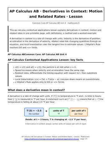
A derivative is a rate of change with units. If \(T(t)\) is temperature in °F and \(t\) is time in hours, then \(T^{\prime}(t)\) is measured in °F per hour. A statement such as \(T^{\prime}(3)=-2.5\) means that at \(t=3\) the temperature is falling at about 2.5 °F per hour.
How do position, velocity and acceleration connect?
For a particle on a line with position \(s(t)\), velocity is \(v(t)=s^{\prime}(t)\) and acceleration is \(a(t)=v^{\prime}(t)=s^{\prime\prime}(t)\). The particle is at rest when \(v=0\). It moves right when \(v>0\) and left when \(v< 0\). Speed \(|v|\) increases when \(v\) and \(a\) have the same sign and decreases when they have opposite signs.
Example. If \(s(t)=t^{3}-6t^{2}+9t\), then \(v(t)=3(t-1)(t-3)\) and \(a(t)=6t-12\). At \(t=2\), \(v=-3\) and \(a=0\).
How do you solve a related rates problem?
- Draw a picture and name every changing quantity.
- Write an equation that links the quantities, valid at every moment.
- Differentiate both sides with respect to time \(t\), using the chain rule.
- Substitute the known values after differentiating.
- Solve and state the answer with units.
A 13-foot ladder has its base \(x\) feet from a wall and its top \(y\) feet up. Since \(x^{2}+y^{2}=169\), we get \(x\frac{dx}{dt}+y\frac{dy}{dt}=0\). If \(x=5\), \(y=12\) and \(\frac{dx}{dt}=2\) ft/s, then \(\frac{dy}{dt}=-\frac{5}{12}(2)=-\frac{5}{6}\) ft/s.
What is local linearization?
Near \(x=a\), a differentiable function is close to its tangent line \(L(x)=f(a)+f^{\prime}(a)(x-a)\). For \(f(x)=\sqrt{x}\) at \(a=25\), \(L(x)=5+\frac{1}{10}(x-25)\), so \(\sqrt{26}\approx L(26)=5.1\). Since \(f^{\prime\prime}< 0\), the tangent line lies above the curve and the estimate is slightly too large.
When can you use L’Hôpital’s Rule?
If \(\lim_{x\to c}\frac{f(x)}{g(x)}\) has the form \(\frac{0}{0}\) or \(\frac{\infty}{\infty}\), then the limit equals \(\lim_{x\to c}\frac{f^{\prime}(x)}{g^{\prime}(x)}\) when that limit exists. Check the form first.
For \(\lim_{x\to 0}\frac{1-\cos x}{x^{2}}\) the form is \(\frac{0}{0}\). Then \(\frac{\sin x}{2x}\) is again \(\frac{0}{0}\), and \(\frac{\cos x}{2}\to\frac{1}{2}\).
Derivatives in Context: Motion and Related Rates: frequently asked questions
How do you tell if a particle is speeding up?
Compare the signs of velocity and acceleration. If they match, the speed is increasing. If they are opposite, the speed is decreasing. Check both at the time or on the interval you care about.
What are the steps for a related rates problem?
Draw a picture, write an equation linking the variables, differentiate with respect to time, substitute the known values, and solve for the unknown rate with units. Substitute only after differentiating.
What does a derivative mean in an applied problem?
It is the instantaneous rate of change of the output per unit of input. For example, if C′(100) = 8 dollars per item, the next item costs about $8 to produce.
When does a linear approximation overestimate?
When the function is concave down near the point, the tangent line lies above the graph, so the estimate is too large. When the function is concave up, the estimate is too small.
When can I use L’Hôpital’s Rule?
Use it only when the limit of the quotient has the indeterminate form 0/0 or ∞/∞. First substitute the limit value to check the form, then differentiate numerator and denominator separately.
How to use this ap calculus contextual applications lesson
Use this ap calculus contextual applications lesson before the worksheet, then check what you learned with the quiz.

- Derivatives in Context: Motion and Related Rates worksheet (25 problems)
- Derivatives in Context: Motion and Related Rates quiz (10 questions)
- Derivatives in Context: Motion and Related Rates test (45 minutes)
- Previous lesson: Chain Rule, Implicit Differentiation and Inverse Functions
- Next lesson: Analyzing Functions with Derivatives
See every chapter on the AP Calculus AB math page.