


This ap statistics chi worksheet answer key solves all 24 problems of the chi-square tests for homogeneity and independence worksheet step by step.
Each solution shows the expected counts, the contributions to the statistic, the degrees of freedom, the p-value and a conclusion written in context. Compare your work step by step, and check the rounding of expected counts.
AP Statistics Chi Worksheet Answer Key: problems 1–5
Problem 1: Totals in a two-way table
Add across each row: \(34+21+15=70\) and \(26+29+25=80\).
Add down each column: \(34+26=60\), \(21+29=50\) and \(15+25=40\).
The grand total is \(70+80=150\), and \(60+50+40=150\) agrees.
Row totals 70 and 80; column totals 60, 50 and 40; grand total 150.
Problem 2: One expected count
Use \(E=\frac{\text{row total}\times \text{column total}}{\text{grand total}}\) with row total 70, column total 60 and grand total 150.
\(E=\frac{70\times 60}{150}=\frac{4200}{150}=28\).
Check: the seventh-grade bus cell is \(\frac{80\times 60}{150}=32\), and \(28+32=60\).
E = 28 sixth graders.
Problem 3: Degrees of freedom
Use \(df=(r-1)(c-1)\).
- \((3-1)(4-1)=2\times 3=6\)
- \((2-1)(5-1)=1\times 4=4\)
- \((4-1)(4-1)=3\times 3=9\)
- \(3(c-1)=12\) gives \(c-1=4\), so \(c=5\).
(a) 6 (b) 4 (c) 9 (d) 5 columns
Problem 4: Conditional percentages
Divide each count by the sample size of 60.
Chess Club: \(\frac{18}{60}=30\%\). Band: \(\frac{33}{60}=55\%\). Robotics: \(\frac{24}{60}=40\%\).
30%, 55% and 40%; Band has the largest percent.
Problem 5: Homogeneity or independence
- One sample, two variables measured on each adult: independence.
- Separate random samples from four stores, one response variable: homogeneity.
- Random assignment to three treatment groups, one response variable: homogeneity.
AP Statistics Chi Worksheet Answer Key: problems 6–10
Problem 6: Hypotheses for homogeneity
The clubs were sampled separately, so this is a test for homogeneity.
\(H_{0}\): The distribution of bike ownership is the same for Chess Club, Band and Robotics members.
\(H_{a}\): The distribution of bike ownership is not the same for at least one of the three clubs.
Problem 7: Hypotheses for independence
- \(H_{0}\): Grade level and favorite sport are independent for students at this school. \(H_{a}\): Grade level and favorite sport are associated for students at this school.
- There are 4 rows and 3 columns, so \(df=(4-1)(3-1)=3\times 2=6\).
df = 6
Problem 8: Expected counts for a 2 by 2 table
Row totals are 80 and 80; column totals are 75 and 85; the grand total is 160.
\(E_{11}=\frac{80\times 75}{160}=37.5\), \(E_{12}=\frac{80\times 85}{160}=42.5\), \(E_{21}=\frac{80\times 75}{160}=37.5\), \(E_{22}=\frac{80\times 85}{160}=42.5\).
Expected: 37.5, 42.5 (morning); 37.5, 42.5 (afternoon).
Problem 9: Contribution of a cell
Use \(\frac{(O-E)^{2}}{E}\).
First cell: \(\frac{(45-37.5)^{2}}{37.5}=\frac{56.25}{37.5}=1.5\).
Second cell: \(\frac{(35-42.5)^{2}}{42.5}=\frac{56.25}{42.5}\approx 1.324\).
1.5 and about 1.324
Problem 10: Chi-square statistic, 2 by 2
Expected counts are 37.5, 42.5, 37.5 and 42.5.
| Contribution | Produce | Baked goods |
|---|---|---|
| Morning | 1.5 | 1.324 |
| Afternoon | 1.5 | 1.324 |
The contributions are 1.5, 1.324, 1.5 and 1.324, so \(\chi^{2}\approx 5.647\).
\(df=(2-1)(2-1)=1\), and the area to the right of 5.647 is \(p\approx 0.0175\).
\(\chi^{2}\) ≈ 5.647, df = 1, p ≈ 0.0175
AP Statistics Chi Worksheet Answer Key: problems 11–15
Problem 11: Chi-square statistic, 2 by 3
Contributions, row by row: sixth grade \(\frac{(34-28)^{2}}{28}\approx 1.286\), \(\frac{(21-23.33)^{2}}{23.33}\approx 0.233\), \(\frac{(15-18.67)^{2}}{18.67}\approx 0.720\).
Seventh grade \(\frac{(26-32)^{2}}{32}=1.125\), \(\frac{(29-26.67)^{2}}{26.67}\approx 0.204\), \(\frac{(25-21.33)^{2}}{21.33}\approx 0.630\).
The sum is \(\chi^{2}\approx 4.199\). Here \(df=(2-1)(3-1)=2\) and \(p\approx 0.1225\).
\(\chi^{2}\) ≈ 4.199, df = 2, p ≈ 0.1225
Problem 12: From statistic to p-value
- The area to the right of 7.82 for 3 degrees of freedom is \(p\approx 0.0499\). This is just below 0.05, so reject \(H_{0}\). (A table agrees: the 0.05 critical value for 3 df is 7.815, and 7.82 is slightly larger.)
- The area to the right of 4.10 for 4 degrees of freedom is \(p\approx 0.3926\), which is greater than 0.05, so fail to reject \(H_{0}\).
(a) p ≈ 0.0499, reject (b) p ≈ 0.3926, fail to reject
Problem 13: Large counts condition
Row totals: 20 and 15. Column totals: 21, 5 and 9. Grand total: 35.
Morning: \(\frac{20\times 21}{35}=12\), \(\frac{20\times 5}{35}\approx 2.857\), \(\frac{20\times 9}{35}\approx 5.143\).
Evening: \(\frac{15\times 21}{35}=9\), \(\frac{15\times 5}{35}\approx 2.143\), \(\frac{15\times 9}{35}\approx 3.857\).
Three expected counts (2.857, 2.143 and 3.857) are less than 5.
The condition does not hold, so a chi-square test is not appropriate.
Problem 14: Conclusion for homogeneity
Compare the p-value with the significance level: \(0.0201\) is less than \(0.05\).
Reject \(H_{0}\). There is convincing evidence that the distribution of bike ownership is not the same for all three clubs.
Problem 15: Conclusion for independence
\(df=(5-1)(2-1)=4\). The area to the right of 5.2 for 4 degrees of freedom is \(p\approx 0.267\).
Because 0.267 is greater than 0.05, fail to reject \(H_{0}\). There is not convincing evidence of an association between age group and preferred pizza topping among these adults.
AP Statistics Chi Worksheet Answer Key: problems 16–20
Problem 16: Largest contribution
Each row total is 100 and the column totals are 170 and 130, so the expected counts are \(\frac{100\times 170}{300}\approx 56.67\) for tea and \(\frac{100\times 130}{300}\approx 43.33\) for coffee in every region.
| Contribution | Tea | Coffee |
|---|---|---|
| North | 4.902 | 6.41 |
| South | 0.049 | 0.064 |
| West | 5.931 | 7.756 |
The sum is \(\chi^{2}\approx 25.113\) with \(df=2\).
West, Coffee contributes the most (about 7.756). Its observed count 25 is below the expected 43.33.
Problem 17: Doubling every count
Doubling every observed count also doubles every expected count, and each term \(\frac{(O-E)^{2}}{E}\) doubles: \(\frac{(2O-2E)^{2}}{2E}=2\cdot\frac{(O-E)^{2}}{E}\).
So \(\chi^{2}=2\times 5.647\approx 11.294\). Check: expected counts are 75 and 85, and the contributions are 3, 2.647, 3 and 2.647, which sum to 11.294.
The degrees of freedom stay at 1, and the p-value falls from 0.0175 to \(p\approx 0.0008\).
\(\chi^{2}\) ≈ 11.294; p ≈ 0.0008 (much smaller)
Problem 18: Working backward from totals
- \(E=\frac{80\times 60}{200}=24\)
- \(\frac{(33-24)^{2}}{24}=\frac{81}{24}=3.375\)
- \(18=\frac{72\times \text{column total}}{240}\), so the column total is \(\frac{18\times 240}{72}=60\).
(a) 24 (b) 3.375 (c) 60
Problem 19: Critical values
- 14.2 is greater than 13.277, so the p-value is less than 0.01: reject \(H_{0}\).
- 5.2 is less than 5.991, so the p-value is greater than 0.05: fail to reject \(H_{0}\).
Check with software: \(p(14.2,\,4)\approx 0.0067\) and \(p(5.2,\,2)\approx 0.0743\).
(a) reject (b) fail to reject
Problem 20: Interpreting a p-value
If time of day and type of first purchase were independent among all shoppers at this market, there would be about a 1.75% chance of getting a sample with a chi-square statistic of 5.647 or larger just from random sampling.
It is not the probability that the null hypothesis is true.
AP Statistics Chi Worksheet Answer Key: problems 21–24
Problem 21: Association is not causation
The teens were sampled, not assigned to sleep amounts, so this is an observational study. Other variables, such as study habits or after-school jobs, may be related to both sleep and grades.
To support a cause-and-effect conclusion, randomly assign volunteers to different required sleep schedules, then compare grade outcomes across the treatment groups with a chi-square test for homogeneity.
Problem 22: Complete test of independence
State. \(H_{0}\): Age group and main news source are independent in this city’s adult population. \(H_{a}\): Age group and main news source are associated. Use \(\alpha=0.05\).
Plan. Chi-square test for independence. Random: the sample is a random sample of adults. The sample of 210 is less than 10% of the more than 100,000 adults. Large counts: every expected count is at least 5 (the smallest is 20).
Do. Expected counts use \(E=\frac{\text{row total}\times \text{column total}}{\text{grand total}}\). Observed counts, with expected counts in parentheses:
| Age group | TV | Online | |
|---|---|---|---|
| 18 to 34 | 22 (20) | 31 (25) | 17 (25) |
| 35 to 54 | 28 (20) | 19 (25) | 23 (25) |
| 55 and up | 10 (20) | 25 (25) | 35 (25) |
The cell contributions \(\frac{(O-E)^{2}}{E}\) are 0.2, 1.44, 2.56, 3.2, 1.44, 0.16, 5, 0, 4. Their sum is \(\chi^{2}=18\). With \(df=(3-1)(3-1)=4\), the p-value is \(p=0.0012\).
Conclude. Because the p-value (0.0012) is less than \(\alpha=0.05\), reject \(H_{0}\). There is convincing evidence that age group and main news source are associated among adults in this city.
\(\chi^{2}\) = 18, df = 4, p ≈ 0.0012: convincing evidence of an association.
Problem 23: Complete test of homogeneity
State. \(H_{0}\): The distribution of satisfaction is the same at all four locations. \(H_{a}\): The distribution of satisfaction is not the same at all four locations. Use \(\alpha=0.05\).
Plan. Chi-square test for homogeneity. Random: there are four separate random samples of diners. Each sample of 80 is less than 10% of the diners at its location (assuming each location serves more than 800 diners). Large counts: every expected count is at least 5 (the smallest is 22.25).
Do. Expected counts use \(E=\frac{\text{row total}\times \text{column total}}{\text{grand total}}\). Observed counts, with expected counts in parentheses:
| Response | Downtown | Mall | Airport | Suburb |
|---|---|---|---|---|
| Satisfied | 62 (57.75) | 55 (57.75) | 48 (57.75) | 66 (57.75) |
| Not satisfied | 18 (22.25) | 25 (22.25) | 32 (22.25) | 14 (22.25) |
The cell contributions \(\frac{(O-E)^{2}}{E}\) are 0.313, 0.131, 1.646, 1.179, 0.812, 0.34, 4.272, 3.059. Their sum is \(\chi^{2}\approx 11.752\). With \(df=(2-1)(4-1)=3\), the p-value is \(p=0.0083\).
Conclude. Because the p-value (0.0083) is less than \(\alpha=0.05\), reject \(H_{0}\). There is convincing evidence that the proportion of satisfied diners is not the same at all four locations.
\(\chi^{2}\) ≈ 11.752, df = 3, p ≈ 0.0083: convincing evidence that satisfaction differs.
Problem 24: Test for an experiment
State. \(H_{0}\): The distribution of outcomes (improved or no change) is the same for all three plans. \(H_{a}\): The distribution of outcomes is not the same for all three plans. Use \(\alpha=0.05\).
Plan. Chi-square test for homogeneity. Random: patients were randomly assigned to the three plans. Large counts: every expected count is at least 5 (the smallest is 18.67).
Do. Expected counts use \(E=\frac{\text{row total}\times \text{column total}}{\text{grand total}}\). Observed counts, with expected counts in parentheses:
| Therapy | Improved | No change |
|---|---|---|
| Plan A | 28 (21.333) | 12 (18.667) |
| Plan B | 22 (21.333) | 18 (18.667) |
| Plan C | 14 (21.333) | 26 (18.667) |
The cell contributions \(\frac{(O-E)^{2}}{E}\) are 2.083, 2.381, 0.021, 0.024, 2.521, 2.881. Their sum is \(\chi^{2}\approx 9.911\). With \(df=(3-1)(2-1)=2\), the p-value is \(p=0.0070\).
Conclude. Because the p-value (0.0070) is less than \(\alpha=0.05\), reject \(H_{0}\). There is convincing evidence that the plans do not all have the same distribution of outcomes.
Because patients were randomly assigned, the difference in outcomes can be attributed to the plans.
\(\chi^{2}\) ≈ 9.911, df = 2, p ≈ 0.0070: reject \(H_{0}\); yes, cause and effect is supported.
How to use this ap statistics chi worksheet answer key
Read this ap statistics chi worksheet answer key after trying each problem yourself, and redo any problem you missed.

Printable PDF · Worksheet Answer Key
AP Statistics Chi-Square Tests for Homogeneity and Independence worksheet answer key
Download the PDF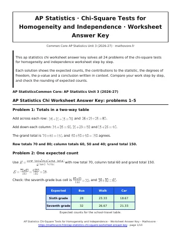
See every chapter on the AP Statistics math page.